Robotics & AI/Google
Google ML crash course (6)
생각하는 이상훈
2023. 2. 27. 12:46
728x90
Linear regression(2)
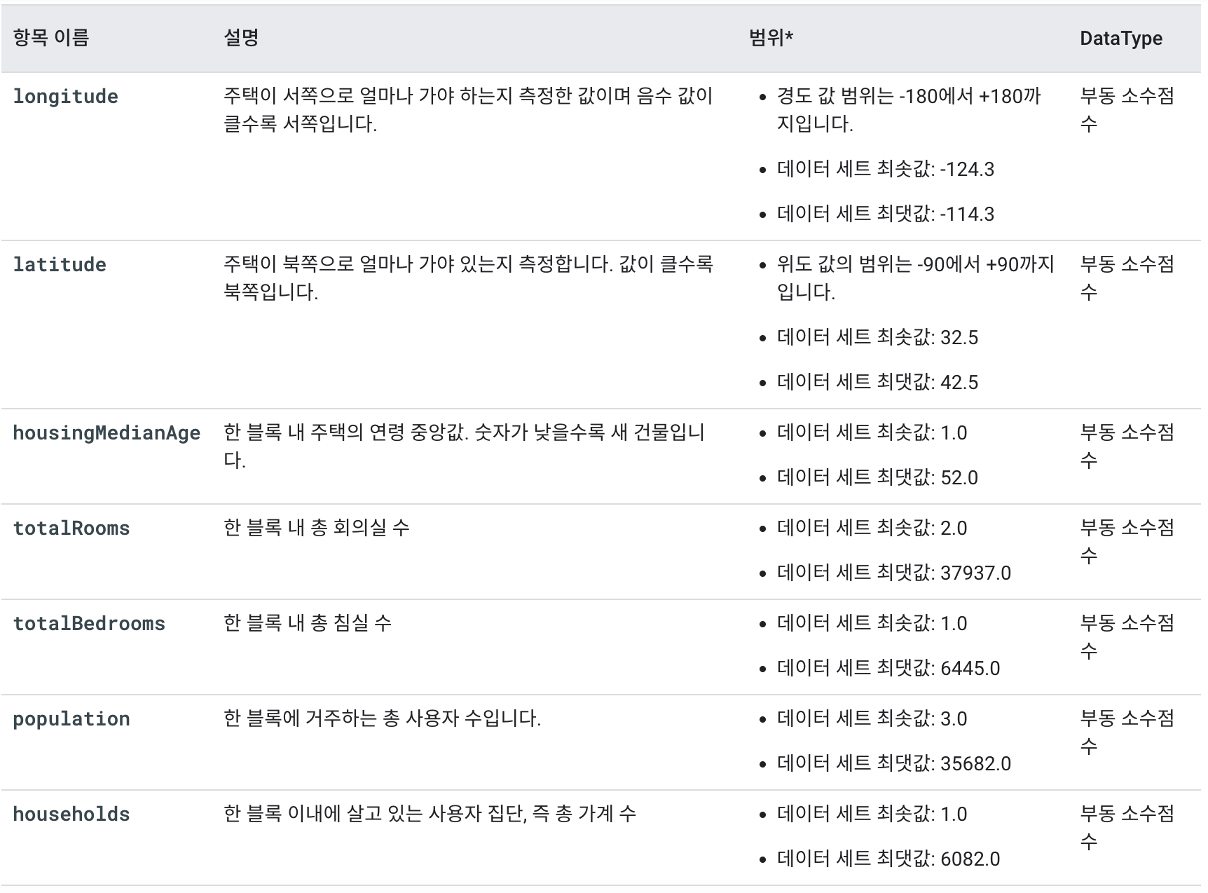
이번에는 실제 데이터셋을 이용해보고자 한다.
캘리포니아의 집값에 대한 데이터셋을 이용하여 선형회귀 과정을 밟아보자.
#@title Import relevant modules
import pandas as pd
import tensorflow as tf
from matplotlib import pyplot as plt

# The following lines adjust the granularity of reporting.
pd.options.display.max_rows = 10
pd.options.display.float_format = "{:.1f}".format
머신러닝에서 csv파일을 이용하는데 csv파일이란 Comma-seperated values 파일로 콤마로 구분하여 데이터셋을 구성한 파일이다.
아래와 같은 구성이다.
"longitude","latitude","housing_median_age","total_rooms","total_bedrooms","population","households","median_income","median_house_value"
-114.310000,34.190000,15.000000,5612.000000,1283.000000,1015.000000,472.000000,1.493600,66900.000000
-114.470000,34.400000,19.000000,7650.000000,1901.000000,1129.000000,463.000000,1.820000,80100.000000
-114.560000,33.690000,17.000000,720.000000,174.000000,333.000000,117.000000,1.650900,85700.000000
-114.570000,33.640000,14.000000,1501.000000,337.000000,515.000000,226.000000,3.191700,73400.000000
csv 파일을 Pandas dataframe에 담는 과정이다.
# Import the dataset.
training_df = pd.read_csv(filepath_or_buffer="https://download.mlcc.google.com/mledu-datasets/california_housing_train.csv")

# Scale the label.
training_df["median_house_value"] /= 1000.0

# Print the first rows of the pandas DataFrame.
training_df.head()
# Get statistics on the dataset.
training_df.describe()임의로 초기화된 모델을 빌드하는 build_model(my_learning_rate),
전달한 examples(feature and label)에서 model을 training하는 train_model(model, feature, labe, epochs)
#@title Define the functions that build and train a model
def build_model(my_learning_rate):
  """Create and compile a simple linear regression model."""
  # Most simple tf.keras models are sequential.
  model = tf.keras.models.Sequential()

  # Describe the topography of the model.
  # The topography of a simple linear regression model
  # is a single node in a single layer.
  model.add(tf.keras.layers.Dense(units=1,
                                  input_shape=(1,)))

  # Compile the model topography into code that TensorFlow can efficiently
  # execute. Configure training to minimize the model's mean squared error.
  model.compile(optimizer=tf.keras.optimizers.experimental.RMSprop(learning_rate=my_learning_rate),
                loss="mean_squared_error",
                metrics=[tf.keras.metrics.RootMeanSquaredError()])

  return model


def train_model(model, df, feature, label, epochs, batch_size):
  """Train the model by feeding it data."""

  # Feed the model the feature and the label.
  # The model will train for the specified number of epochs.
  history = model.fit(x=df[feature],
                      y=df[label],
                      batch_size=batch_size,
                      epochs=epochs)

  # Gather the trained model's weight and bias.
  trained_weight = model.get_weights()[0]
  trained_bias = model.get_weights()[1]

  # The list of epochs is stored separately from the rest of history.
  epochs = history.epoch

  # Isolate the error for each epoch.
  hist = pd.DataFrame(history.history)

  # To track the progression of training, we're going to take a snapshot
  # of the model's root mean squared error at each epoch.
  rmse = hist["root_mean_squared_error"]

  return trained_weight, trained_bias, epochs, rmse

print("Defined the build_model and train_model functions.")
plotting함수를 정의한다.
#@title Define the plotting functions
def plot_the_model(trained_weight, trained_bias, feature, label):
  """Plot the trained model against 200 random training examples."""

  # Label the axes.
  plt.xlabel(feature)
  plt.ylabel(label)

  # Create a scatter plot from 200 random points of the dataset.
  random_examples = training_df.sample(n=200)
  plt.scatter(random_examples[feature], random_examples[label])

  # Create a red line representing the model. The red line starts
  # at coordinates (x0, y0) and ends at coordinates (x1, y1).
  x0 = 0
  y0 = trained_bias
  x1 = random_examples[feature].max()
  y1 = trained_bias + (trained_weight * x1)
  plt.plot([x0, x1], [y0, y1], c='r')

  # Render the scatter plot and the red line.
  plt.show()


def plot_the_loss_curve(epochs, rmse):
  """Plot a curve of loss vs. epoch."""

  plt.figure()
  plt.xlabel("Epoch")
  plt.ylabel("Root Mean Squared Error")

  plt.plot(epochs, rmse, label="Loss")
  plt.legend()
  plt.ylim([rmse.min()*0.97, rmse.max()])
  plt.show()

print("Defined the plot_the_model and plot_the_loss_curve functions.")
call the model functions
# The following variables are the hyperparameters.
learning_rate = 0.01
epochs = 30
batch_size = 30

# Specify the feature and the label.
my_feature = "total_rooms"  # the total number of rooms on a specific city block.
my_label="median_house_value" # the median value of a house on a specific city block.
# That is, you're going to create a model that predicts house value based
# solely on total_rooms.

# Discard any pre-existing version of the model.
my_model = None

# Invoke the functions.
my_model = build_model(learning_rate)
weight, bias, epochs, rmse = train_model(my_model, training_df,
                                         my_feature, my_label,
                                         epochs, batch_size)

print("\nThe learned weight for your model is %.4f" % weight)
print("The learned bias for your model is %.4f\n" % bias )

plot_the_model(weight, bias, my_feature, my_label)
plot_the_loss_curve(epochs, rmse)
예측을 위한 model을 구성한다.
def predict_house_values(n, feature, label):
  """Predict house values based on a feature."""

  batch = training_df[feature][10000:10000 + n]
  predicted_values = my_model.predict_on_batch(x=batch)

  print("feature   label          predicted")
  print("  value   value          value")
  print("          in thousand$   in thousand$")
  print("--------------------------------------")
  for i in range(n):
    print ("%5.0f %6.0f %15.0f" % (training_df[feature][10000 + i],
                                   training_df[label][10000 + i],
                                   predicted_values[i][0] ))
predict_house_values(10, my_feature, my_label)다른 feature를 추가해본다.
#@title Double-click to view a possible solution.

my_feature = "population" # Pick a feature other than "total_rooms"

# Possibly, experiment with the hyperparameters.
learning_rate = 0.05
epochs = 18
batch_size = 3

# Don't change anything below.
my_model = build_model(learning_rate)
weight, bias, epochs, rmse = train_model(my_model, training_df,
                                         my_feature, my_label,
                                         epochs, batch_size)

plot_the_model(weight, bias, my_feature, my_label)
plot_the_loss_curve(epochs, rmse)

predict_house_values(10, my_feature, my_label)
define a synthetic feature
#@title Double-click to view a possible solution to Task 4.

# Define a synthetic feature
training_df["rooms_per_person"] = training_df["total_rooms"] / training_df["population"]
my_feature = "rooms_per_person"

# Tune the hyperparameters.
learning_rate = 0.06
epochs = 24
batch_size = 30

# Don't change anything below this line.
my_model = build_model(learning_rate)
weight, bias, epochs, mae = train_model(my_model, training_df,
                                        my_feature, my_label,
                                        epochs, batch_size)

plot_the_loss_curve(epochs, mae)
predict_house_values(15, my_feature, my_label)
728x90